Contribution Templates

18 minute(s) read

Creating Contribution Templates #

Contribution templates define the content and appearance of input forms for Contribution Campaigns.

Contribution starts with one or more planning report spreadsheets, which might normally be distributed using Reportworq. You can turn the reports into Contribution templates by adding one or more formulas that define the input ranges that require data entry. You can also add filters, checkboxes, picklists, and data validation formulas with associated warning messages.

This article describes how to use the Reportworq add-in for Excel to create formulas for Contribution templates. Alternatively, you can create and edit the formulas manually.

The main topics in this article are as follows:

When you are finished configuring your Contribution template, set the spreadsheet’s Print Area to include only the cells you want Contribution users to see. Save the Contribution template file in a location that is designated as a Report Provider.

Accessing the Reportworq Add-in #

Before you can use the add-in for the first time, you must install it. Each time you use the add-in, you must launch it. To install or launch the add-in, a Reportworq license is required.

Internet access is required to install or use the Reportworq add-in.

To launch the add-in after it has been installed:

Open the Excel report (.xlsx file) you want to modify.
At the top of Excel, select the Reportworq tab and then select the Reportworq open button.

If you are not logged in to Reportworq, the login prompt appears.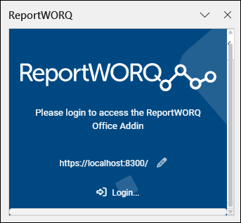
If the login prompt appears, do the following:
- If Reportworq uses a port number other than 8300, or Reportworq is installed on a different computer, Select the edit icon , provide the correct URL for accessing Reportworq, and then select View.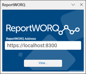
- Select Login, provide your User Name and Password as prompted, and then select Login.
  The Reportworq task pane appears.

Opening Reports Previously Modified by the Add-in #

If you open a report that has been previously modified by the Reportworq add-in, Excel automatically attempts to launch the add-in:

If the add-in is installed but you are not logged in to Reportworq, you are prompted to log in.
If the add-in is not installed, you are prompted to Accept and Continue, and then you are prompted to log in to Reportworq.

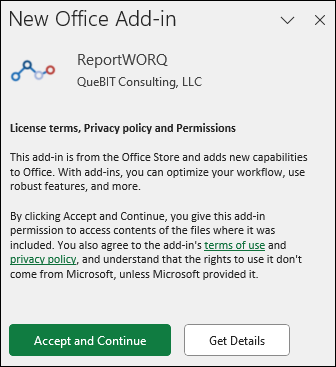
After you log in, the Reportworq add-in pane appears.

View and Create Input Ranges #

You can create new input formulas or review and modify existing ones. When you select View and Create Input Ranges, the Edit Input Formulas area appears.

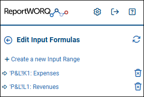
To create or modify an input range:

If you are modifying an existing input formula, select it from the list, and proceed to Step 4.
Select Create a new Input Range.
The Select Data box appears.
Select or specify which empty cell in the spreadsheet will contain the new input formula.
Tip: Do not place an input formula in a column that contains row headers, or in a row that contains column headers.
Configure the properties of the input range:

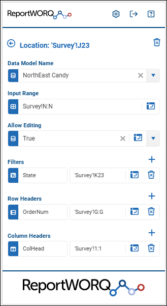
Location — The cell that contains the input formula. The Location cell displays the Data Model Name.
Tip: Do not place an input formula in a column that contains row headers, or in a row that contains column headers.
Data Model Name — References the data model that contains all collected data for the input range.
Input Range — The range of cells to be made editable by Contributors. You can type a cell range reference or select the icon and then drag to select. If you want to define an input range that includes multiple blocks of cells, enter the RW.INPUT formula manually, setting the inputRange argument to specify multiple cell ranges, for example, (D4:D6,D9:D11,F4:G6,F9:G11). For more information, see RW.INPUT Function.
Note: The input range cannot include Excel control cells, such as ones that contain formulas for filters, checkboxes, or picklists.
Allow Editing — Controls whether Contributors can edit data in the input cell(s).
When True, Contributors can edit the input cell(s). When False, they cannot. This setting is True by default.
Tip: If you want to gather data that is the result of a formula, place the formula in an input cell and set Allow Editing to FALSE so Contributors cannot overwrite it. The calculated result of the formula will be included as Contribution input.
Filters — Defines filters in the data model. Filters further define the context of the data that is represented by the row/column intersection and are often used for bursting input forms. They are generally placed at the top left of an input form as a summary of the “slice” or “context” of the data. For example, if sales data has salesperson names on rows and months on columns, a region filter could be used to burst out one iteration of the input form per sales region. On each region’s input form, the sales region name would appear in the cell where the filter is located.
To define a filter, specify a field name to be used in the data model and select a single cell to contain the filter. There can be zero or more filters.
Row Headers — Defines rows in the data model. Specify a field name and select a single column that contains the row headers. You can type a cell reference or select the icon and then select any cell in the column. There can be one or more Row Headers.
Column Headers — Defines columns in the data model. Specify a field name and select a single row that contains the column headers. You can type a cell reference or select the icon and then select any cell in the row. There can be one or more Column Headers.

Tip: If you select a box that contains a cell reference, the cells are highlighted in the spreadsheet view.

Manage Validation Formulas #

Validations test cell values and display messages to Contributors and Approvers if test results are FALSE. You can set up any number of validations for a given cell and can apply the validation message to any cell you specify. On Reportworq Contribution input forms in Webview, validation messages appear as cell comments and are listed on the Validations tab of the Details pane.

When you select Manage Validation Formulas, the Edit Validation Formulas area appears. You can create new validations or review and modify existing ones. As you hover over each validation in the list, the cell that is informed by the validation is highlighted in the spreadsheet.

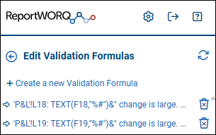
To create or modify a validation formula:

If you are modifying an existing validation formula, select it from the list, and proceed to Step 4.
Select Create a new Validation Formula.
The Select Data box appears.
Select or specify which empty cell in the spreadsheet will contain the new validation formula. This is the Location.
Tip: Do not place a validation formula in a column that contains row headers, or in a row that contains column headers.
Configure the properties of the validation, as follows:

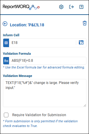
Location – The cell that contains the validation formula. The Location cell always displays the current test result (TRUE or FALSE).
Tip: Do not place a validation formula in a column that contains row headers, or in a row that contains column headers.
Inform Cell — The cell to which the validation message is applied if the validation test result is FALSE.
You can type a cell reference or select the icon and then select the cell.
Validation Formula — The formula that tests the cell value. You can use cell references and Excel functions in the formula.
The validation test runs whenever the cell value changes. If the test result is FALSE, the validation message is activated.
Validation Message — The message text that appears as a cell comment in the Inform Cell if the test result is FALSE. On Reportworq Contribution input forms in Webview, validation messages appear as cell comments and are listed on the Validations tab of the Details pane.
Require Validation for Submission — Select this checkbox to block the submission of data that does not meet validation requirements.

Tip: If you select a box that contains a cell reference, the cells are highlighted in the spreadsheet view.

Manage Filter Formulas #

The Filter formula defines a row filter that appears on the input form as a dropdown list. Contributors and Approvers can apply these filters to view a subset of rows. Multiple filter criteria can be selected.

As in Excel, filters include a Search box. When search criteria are applied, the filter’s Select All option changes to Select All Selected, which selects all the results of the search.

To define a filter, you specify the filter Location cell that contains the filter formula, a label for that cell (optional), and the filter range (optional). The filter range contains the filter criteria (selectable values to filter on), and is a contiguous block of cells from a single column. If you do not specify a filter range, the range extends from the filter Location cell downwards until an empty cell is encountered.

When you select Manage Filter Formulas, the Edit Filter Formulas area appears. You can create new filters or review and modify existing ones.

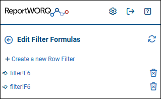
To create or modify a filter formula:

If you are modifying an existing filter formula, select it from the list and proceed to Step 4.
Select Create a new Row Filter.
The Select Data box appears.
Select or specify an empty cell to contain the filter formula. This cell is the filter Location.
Configure the properties of the filter formula, as follows:

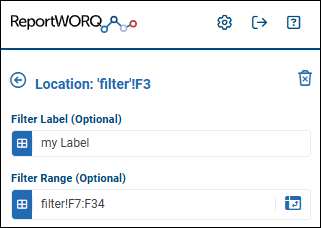
If you want the cell that contains the filter to display a label, type the label text in the Filter Label box.
To define the filter range, do one of the following:
- To define the exact filter range: In the Filter Range box, specify a contiguous block of cells from a single column.
  You can type a cell range reference or select the icon and then select the cells.
- To define the filter range as a block of cells immediately below the filter location: Leave the Filter Range box blank.
  The filter range extends from the filter Location cell downwards until an empty cell is encountered.

Tip: If you select a box that contains a cell reference, the cells are highlighted in the spreadsheet view.

Manage Checkbox Formulas #

The Checkbox formula adds a checkbox to the input form. Contribution users can select or clear the checkbox, which is clear by default.

When you select Manage Checkbox Formulas, the Edit Checkbox Formulas area appears. You can define new checkboxes or review and modify existing ones.

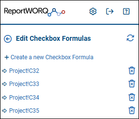
To create or modify a checkbox formula:

If you are modifying an existing checkbox formula, select it from the list and proceed to Step 4.
Select Create a new Checkbox Formula.
The Select Data box appears.
Select or specify an empty cell to contain the checkbox formula. This cell is the checkbox Location.
Configure the properties of the checkbox formula, as follows:

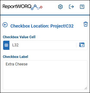
In the Checkbox Value Cell box, specify which cell receives the checkbox value.
When a Contribution user selects or clears the checkbox, the Checkbox Value Cell receives the checkbox value, which is TRUE if the checkbox is selected and FALSE if it is cleared.
You can type a cell reference or select the icon and then select the cell.
If you want a text label to be displayed beside the checkbox, type the label text in the Checkbox Label box.

Tip: If you select a box that contains a cell reference, the cells are highlighted in the spreadsheet view.

Manage Picklist Formulas #

The Picklist formula adds a dropdown picklist to the input form. Contribution users can select one value from the picklist.

When you select Manage Picklist Formulas, the Edit Picklist Formulas area appears. You can define new picklists or review and modify existing ones.

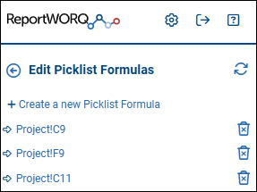
To create or modify a picklist formula:

If you are modifying an existing picklist formula, select it from the list and proceed to Step 4.
Select Create a new Picklist Formula.
The Select Data box appears.
Select or specify an empty cell to contain the picklist formula. This cell is the picklist Location.
Configure the properties of the picklist formula, as follows:

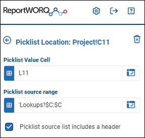
In the Picklist Value Cell box, specify which cell receives the value selected by the Contribution user.
You can type a cell reference or select the icon and then select the cell.
In the Picklist source range box, specify a cell range that contains the values to appear in the picklist. The cell range must be within a single column.
Select Picklist source contains a header if you do not want to the first value from the Picklist source range to be included in the picklist.

Tip: If you select a box that contains a cell reference, the cells are highlighted in the spreadsheet view.

Preview the Input Form #

You can preview the input form and interact with it, to ensure that it appears as you want it to.

Before you preview the input form, set the spreadsheet’s Print Area to include only the cells you want Contribution users to see.

Manage Settings #

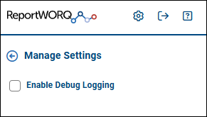
When you select Manage Settings , the following settings appear:

Enable Debug Logging – If selected, Reportworq creates a detailed activity log that Reportworq Technical Support can use to diagnose problems. Enable this option only if requested to do so by Technical Support.

Excel Features and Formatting #

Contribution supports most Excel features. Most Excel formatting options persist when the Contribution template is later used to create input forms. This topic highlights selected Excel features and formatting options, and provides information about how they can affect input forms.

Excel Features:

Arrow keys and scrolling — Contribution input forms support the use of arrow keys (up, down, left, right). Scroll bars appear if the input form is too large to display in the browser window.

Excel Formatting Options:

Filters — If you apply Excel data filters, the input form will include only the rows that are not hidden by the filters.
Alternatively, you can use the Reportworq add-in to create filters that Contributors and Approvers can apply.
Freeze Panes — Freeze pane settings in Contribution templates persist in input forms. If merged cells span across a freeze-pane border, they are anchored to the frozen pane.
Groups — You can include grouped rows and columns in Contribution templates. Contributors and Approvers can expand and collapse groups, in both the Reportworq web view and input forms that have been downloaded for offline editing.
If the print area is set and a group spans across the print area boundary, only the cells within the print area are included on input forms. If the group contains a chart that spans across the print area boundary, the entire chart is included.
Print Area — Template creators can set the print area to define which cells are included on input forms:
- If the print area is set — Only cells within the print area are included, even if they belong to a cell group that extends beyond the print area. If a chart spans across the print area boundary, the entire chart is included.
- If the print area is not set — Input forms include a rectangular block of cells containing all non-empty cells. If the worksheet includes grouped rows or columns, the entire group is included, even if the group contains empty rows or columns.
Sparklines — Sparkline charts are supported in Contribution input forms. If the data range for a sparkline includes input cells, the sparkline chart updates whenever a Contributor or Approver changes the value of any such cell.

Reminder: When you are finished configuring your Contribution template, set the spreadsheet’s Print Area to include only the cells you want Contribution users to see. Save the Contribution template file in a location that is designated as a Report Provider.

Create and Edit Formulas Manually #

As an alternative to using the Reportworq Excel add-in, you can use Reportworq functions to create formulas for Contribution templates.

Important: Do not place formulas in rows that have column headers or in columns that have row headers.

This topic describes the following Reportworq functions for Contribution templates:

RW.CONTRIBUTION.Check Function — Defines a data validation test and a result message.
RW.CONTRIBUTION.CHECKBOX Function — Adds a checkbox, which Contribution users can select or clear.
RW.CONTRIBUTION.FILTER Function — Defines a row filter that Contribution users can apply, to view a subset of rows on the input form.
RW.CONTRIBUTION.INPUT Function — Defines an input range, where Contribution users can provide data.
RW.CONTRIBUTION.LIST Function — Defines a dropdown picklist from which Contribution users can select a value.

RW.Contribution.Check #

RW.Contribution.Check aka RW.Check adds a validation rule for a contribution cell and optionally marks that rule as required. If you are on a version earlier than 5.0.0.91 please use RW.Check.

Syntax #

=RW.Contribution.Check(targetCell, validationPassed, validationMessage, [validationRequired])

Arguments #

#	Name	Type	Default	Description
1	`targetCell`	Cell reference	(required)	Contribution cell being validated.
2	`validationPassed`	Boolean	(required)	Validation expression result.
3	`validationMessage`	String	(required)	Message shown to the user when the rule fails.
4	`validationRequired`	Boolean	`FALSE`	When `TRUE`, the validation is required rather than advisory.

Behavior #

The formula stores the target cell, validation result, message, and required flag for the contribution framework.
The formula cell itself evaluates to the Boolean value of validationPassed.
Multiple RW.Contribution.Check formulas can be collected and shown together during contribution validation.

Usage notes #

Use validationRequired=TRUE for hard-stop rules.
Leave the fourth argument blank when the message should be informational or warning-like.

Examples #

=RW.Contribution.Check(B5, B5>0, "Amount must be greater than zero", TRUE)

=RW.Contribution.Check(C10, LEN(C10)>0, "Description is required")

Common mistakes #

Situation	Result
`targetCell` is not a cell reference	Formula errors during parsing
Fewer than 3 arguments	Formula errors during parsing
Expecting the formula cell to show the message text	The formula cell only evaluates to `TRUE` or `FALSE`

RW.Contribution.Checkbox #

RW.Contribution.Checkbox aka RW.Checkbox creates a checkbox control for a contribution workbook and links it to a target cell. If you are on a version earlier than 5.0.0.91 please use RW.Checkbox.

Syntax #

=RW.Contribution.Checkbox(targetCell, label)

Arguments #

#	Name	Type	Default	Description
1	`targetCell`	Cell reference	(required)	Cell that stores the checkbox result.
2	`label`	String	(required)	Text shown next to the checkbox.

Behavior #

ReportWorq records the target cell coordinates and display label for the control.
The formula cell evaluates to [] label so the control has a visible placeholder in Excel.
Contribution rendering uses the formula metadata to create the interactive checkbox behavior.

Usage notes #

Point targetCell at the cell that should receive the checked/unchecked value.
Pair RW.Contribution.Checkbox with RW.Contribution.Input when the checkbox is part of a larger contribution form.

Examples #

=RW.Contribution.Checkbox(Input!C5, "Include Historical Data")

=RW.Contribution.Checkbox(D10, "Approve for Export")

Common mistakes #

Using a text literal instead of a real target-cell reference.
Expecting the checkbox label cell itself to store the value.

RW.Contribution.Filter #

RW.Contribution.Filter aka RW.Filter defines a contribution filter control and the list of values that control should offer. If you are on a version earlier than 5.0.0.91 please use RW.Filter.

Syntax #

=RW.Contribution.Filter([label], [filterValuesRange])

Arguments #

#	Name	Type	Default	Description
1	`label`	String	`""`	Optional label shown for the filter control.
2	`filterValuesRange`	Single-column range	(auto-detect)	Optional list of filter values.

Behavior #

With 0 arguments, ReportWorq reads the values from the cells directly below the formula until it reaches the first blank cell.
With 1 argument, the label is supplied explicitly but the values are still read from the cells below the formula.
With 2 arguments, the values come from the supplied range, which must be a single column.
The formula cell evaluates to the label text.

Usage notes #

Auto-detect mode is convenient when the filter values already live in the same worksheet column.
Use an explicit range when the values are maintained elsewhere in the workbook.

Examples #

=RW.Contribution.Filter()

=RW.Contribution.Filter("Region")

=RW.Contribution.Filter("Product", Control!B2:B10)

Common mistakes #

Situation	Result
Explicit range spans multiple columns	Formula errors
Expecting auto-detect to skip blanks in the middle	Auto-detect stops at the first blank cell

RW.Contribution.Input #

RW.Contribution.Input aka RW.Input defines the editable range and dimensional context for a contribution form. If you are on a version earlier than 5.0.0.91 please use RW.Input.

Syntax #

=RW.Contribution.Input(inputRange, formName, [allowEditing], fieldName1, fieldReferenceOrValue1, [fieldName2, fieldReferenceOrValue2], ...)

Arguments #

#	Name	Type	Default	Description
1	`inputRange`	Range / multi-range	(required)	Cells that belong to the contribution input area.
2	`formName`	String	(required)	Logical form/model name used to group the inputs.
3	`allowEditing`	Boolean	`TRUE`	Optional edit flag. If omitted, ReportWorq assumes editing is allowed.
4+	`fieldName`, `fieldReferenceOrValue`	Repeating pairs	(optional)	Dimensional context for the input range.

Behavior #

ReportWorq classifies each field reference as a row axis, column axis, filter, or static value.
A single-row range becomes a row axis. A single-column range becomes a column axis. Single cells and rectangular ranges become filters. Literal values become static context values.
Input cells are created only where every referenced field resolves to a non-blank value.
The formula cell is cleared after evaluation.

Usage notes #

Keep the field pairs consistent for every RW.Contribution.Input formula that belongs to the same contribution model.
Use row references, column references, and filter cells deliberately so the dimensional routing is unambiguous.
A rectangular multi-cell range is treated as a filter, not as a row or column axis.

Examples #

=RW.Contribution.Input(D7:F9, "Expenses", TRUE, "Accounts", 6:6, "Products", A:A, "Period", B2)

=RW.Contribution.Input(D7:F9, "Expenses", TRUE, "Period", B2, "Version", B3, "Dept", B4)

=RW.Contribution.Input(D7, "Model", TRUE, "Rows", 1:1, "Cols", A:A)

Common mistakes #

Situation	Result
Fewer than 2 arguments	Formula errors during parsing
Odd number of trailing field/value arguments	The unmatched trailing item is ignored
A required field resolves to blank for a cell in `inputRange`	That input cell is skipped
Treating a multi-row, multi-column rectangle as a row or column axis	ReportWorq treats it as a filter

RW.Contribution.List #

RW.Contribution.List aka RW.List creates a dropdown-style contribution control backed by a list of values. If you are on a version earlier than 5.0.0.91 please use RW.Input.

Syntax #

=RW.Contribution.List(targetCell, listValuesRange, includesHeader)

Arguments #

#	Name	Type	Default	Description
1	`targetCell`	Cell reference	(required)	Cell that should store the selected value.
2	`listValuesRange`	Range	(required)	Range that contains the list options.
3	`includesHeader`	Boolean	(required)	When `TRUE`, the first item is treated as a header rather than an option.

Behavior #

The target cell coordinates are stored for the contribution UI.
ReportWorq reads the values from listValuesRange, removes duplicates, and stores the resulting option list.
When includesHeader=TRUE, the first value becomes the list header and is excluded from the options.
The formula cell evaluates to a readable Picklist: ... summary.

Usage notes #

Use a dedicated control sheet or named range to maintain the list values.
When you want the first value to be a label instead of a choice, set includesHeader to TRUE.

Examples #

=RW.Contribution.List(Input!C5, Control!A1:A20, TRUE)

=RW.Contribution.List(B10, Values!A1:A100, FALSE)

Common mistakes #

Using a text literal instead of a real targetCell reference.
Forgetting that duplicate list values are collapsed into unique options.

Updated on July 17, 2026

Create A Support Ticket

Creating Contribution Templates #

Accessing the Reportworq Add-in #

Opening Reports Previously Modified by the Add-in #

View and Create Input Ranges #

Manage Validation Formulas #

Manage Filter Formulas #

Manage Checkbox Formulas #

Manage Picklist Formulas #

Preview the Input Form #

Manage Settings #

Excel Features and Formatting #

Create and Edit Formulas Manually #

RW.Contribution.Check #

Syntax #

Arguments #

Behavior #

Usage notes #

Examples #

Common mistakes #

RW.Contribution.Checkbox #

Syntax #

Arguments #

Behavior #

Usage notes #

Examples #

Common mistakes #

RW.Contribution.Filter #

Syntax #

Arguments #

Behavior #

Usage notes #

Examples #

Common mistakes #

RW.Contribution.Input #

Syntax #

Arguments #

Behavior #

Usage notes #

Examples #

Common mistakes #

RW.Contribution.List #

Syntax #

Arguments #

Behavior #

Usage notes #

Examples #

Common mistakes #