This article explains how to author Excel source reports using the Reportworq add-in for Excel, based on reporting models created using the Reportworq web interface.

Each Reportworq Distribution Job or Contribution Campaign is based on one or more source reports, which are typically Excel workbook (.xslx) files. Each source report contains one or more individual reports based on reporting models derived from Reportworq datasources such as financial planning systems or other supported databases. Reportworq uses source reports as templates to generate report output for distribution or input forms for Contribution Campaigns.

Report authors can create source reports in Excel, using the Reportworq add-in. All procedures in this article are to be performed in Excel.

Reportworq is designed to support and take full advantage of almost all Excel features, including Microsoft Excel's standard built-in functions. Reportworq additionally supports several data provider-specific Excel functions which are documented, per data provider, in Datasources articles. For more information, see Excel Functions.

For more information on the Reportworq add-in

The main sections of this article are as follows:

• Creating or Opening a Report
• Editing Report Options
• Editing Column Options

Manage Reports Menu#

The Manage Reports menu provides access to report authoring features. It consists of an Actions area and collapsible lists of all reports, sorted by worksheet. In the following example, the source report includes three worksheets named Production, Fulfillment, and Executive.

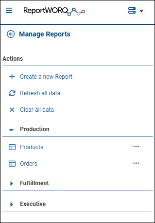
From the Actions area, you can:

• Create a new Report -- Creates a report on the current worksheet.
• Refresh all data -- Renders all reports, using fresh data from their data sources.
• Clear all data -- Deletes data from all reports, leaving the report headings intact.

From the report lists, you can select a report to open it for editing.

Tip: To return to the Manage Reports pane at any time, select the Reportworq logo at the top of the add-in and then select Manage Reports.

Creating or Opening a Report#

A source report (.xlsx file) can contain any number of authored reports, on any number of worksheets. A worksheet can contain multiple reports. After you create a new report, you must edit it to define its contents and properties.

Note: Within this article, authored reports are simply called reports.

Important: Rename Excel worksheets as required before adding reports. Authored reports reference cell locations, which include worksheet names, to position report output.

To create a new report:

1. Navigate to the Excel worksheet where you want to add the new report.
2. From the main menu of the Reportworq add-in, select Manage Reports and then select Create a new Report. The Columns list appears. The list is empty because the report does not yet have a data connection.
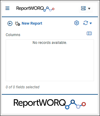
3. Select New Report. An expandable list of reporting models appears. The top-level nodes are datasource names. The second-level nodes indicate the model types. The blue items are individual models.
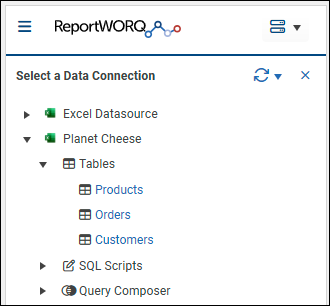
4. Browse to select the reporting model that contains the required data. The Columns list appears.
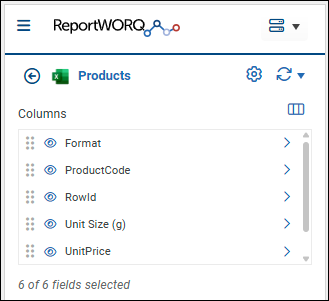
5. Select the fields icon. The Choose Fields list appears.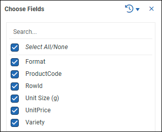
6. Select the fields you need for the report. This includes visible fields as well as hidden fields required for filter queries. Tip: Choosing only the required fields reduces the volume of queries sent to the underlying datasource and improves performance.
7. Close the Choose Fields list (x) to return to the Columns list. The report is ready for editing. Tip: Initially, the report is not displayed on the worksheet. You must refresh the report to preview it.

To open an existing report:

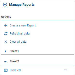
1. From the main menu of the Reportworq add-in, under Reporting, select Manage Reports. 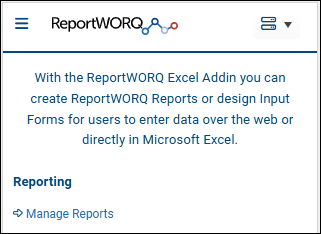The Manage Reports interface appears. Reports are listed, and are grouped by worksheet. In the following example, the Supply Chain worksheet contains two reports named Products and Orders.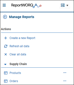
2. If you want to view the report in the spreadsheet as you edit it, open the Excel worksheet tab that contains the report.
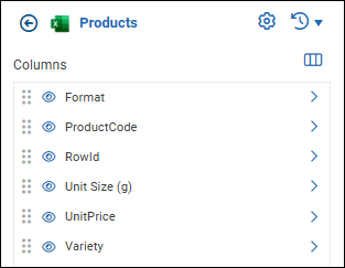
3. Select the report from the list. A list of columns (data fields) appears. The following example shows columns for the Products report. 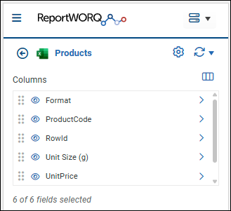Tip: To return to the main menu, select the Back to Reports icon.

Refreshing or Clearing a Report#

When you first create a report, it is not displayed on the worksheet. You must refresh the report to see it. By default, reports are rendered at the top left corner of the worksheet (cell A1). You can change the Location setting on the Import tab of Report Options.

You can refresh a report from cached data or from source data, or clear a report to temporarily delete the data but keep the headings.

You can also send report details to Reportworq Technical Support for analysis.

To refresh a report:

1. Near the top of the authoring interface, select the refresh icon shown ( or ), or expand the refresh menu and select a different refresh option:
2. Refresh from source -- Queries the underlying datasource for fresh data and then renders the report. Tip: The first time you refresh the report, this is the only available option.
3. Refresh from cached data -- Renders the report based on data from the most recent query. This option reduces the volume of queries sent to the datasource, and the report may render more quickly.

To clear a report:

• Expand the refresh menu and then select Clear Report. 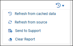All column data is deleted, but the column headers remain visible. The deleted data will be restored upon refresh.

To send report details to Reportworq Technical Support:

• Expand the refresh menu and then select Send to Support.

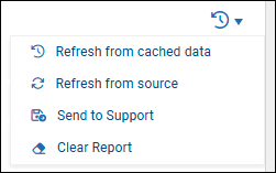
Editing Report Options#

The Report Options area includes settings that apply to the overall report.

To access report options:

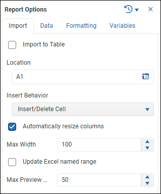
• From the Columns view, select the Report Settings icon. The Report Options area consists of four tabs (Import, Data, Formatting, and Variables).

Note: For options that can be set at both the report level and at the column level, the column level settings override those set at the report level.

Import Tab#

Import tab options control how and where the report is imported into the current worksheet. The Import tab includes the following options:

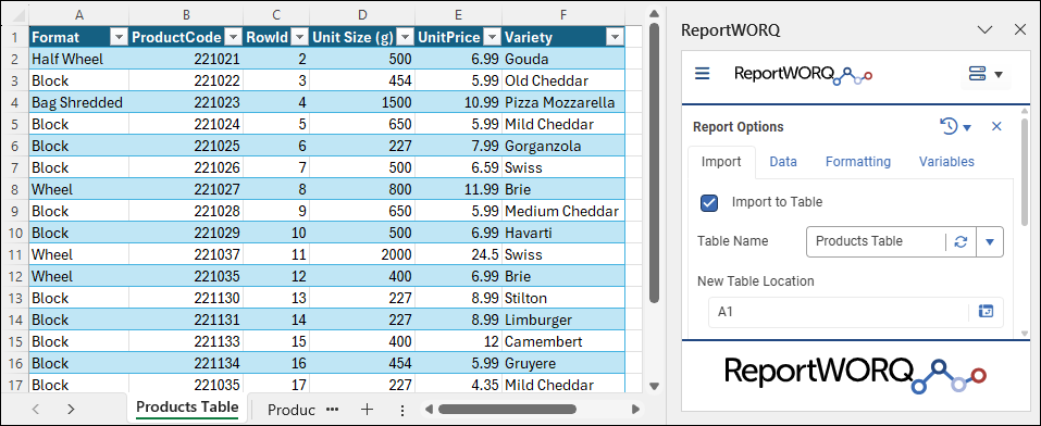
• Import to Table -- When selected, the report output populates an existing Excel table. The table includes filters in each column, which you can apply to limit the data displayed in Reportworq Job output. To configure the table, select the Table Name from the list and specify the New Table Location as a cell or cell range. The top left cell of the table will appear at the specified cell location or the top left cell of the range. In the example below, the table is named Products Table, and it is located at cell A1.

• Location -- Cell or cell range reference that defines the top left corner of the report. If a cell range is specified, the report is aligned with the top left corner of the range.
• Insert Behavior -- Defines how the report is rendered:
  • Overwrite Cells -- The report replaces the contents of the cells where it is rendered. No cells or rows shift. If the number of report rows decreases, excess cells are left blank upon rendering.
  • Insert/Delete Cell -- Initially, the report overwrites the cells where it is rendered. If the number of report rows changes, cells directly below the report shift up or down accordingly upon rendering.
  • Insert/Delete Rows -- Initially, the report overwrites the cells where it is rendered. If the number of report rows changes, rows below the report shift up or down accordingly upon rendering. Cells beside the report also shift up or down, but rows above the report are unaffected.
• Automatically resize columns -- When the report is rendered, column widths adjust to fit their contents.
  • Max Width -- Specify the maximum column width, in pixels.
• Update Excel named range -- When the report is rendered, the specified named range is populated with the report contents. The named range resizes to fit the report contents. Note: This feature takes effect when the report is used in a Reportworq Job, but not when the report shown in Excel is refreshed.
  • Include header row in range -- The header row of the report is included in the named range.
  • Named Range -- The name of the named range. The named range must already exist; Reportworq does not create named ranges.
• Max Preview Rows -- The number of rows to be rendered when the report is refreshed. To show all rows, set Max Preview Rows to Note: This setting does not affect the number of rows rendered when the report runs as part of a Reportworq job.

Data Tab#

• Show totals for aggregate fields -- Enables aggregate totals to be displayed in the report. Aggregate totals can be displayed only for columns that are configured to calculate aggregates, on the Data tab of their Column Options. If any columns in the report are grouped or sectioned, they must also be configured to show totals for aggregate fields, on the Header tab of their Column Options.
• Limit report rows -- When selected, the Row Limit box appears. Specify the maximum number of data rows to be rendered when the report runs as part of a Reportworq Job.
• Filters -- Enables you to define a set of grouped data filters at the report level. Rows that do not meet all filter criteria are excluded from reports.

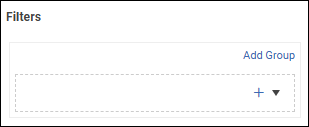
Tip: You can also define filters for individual columns, on the Data tab of their Column Options.

To define report-level filters:

1. In the Filters area of the Data tab, expand the + list and select a column you want to filter. A filter expression box appears. The field name appears above it. 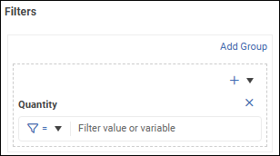Tip: A dashed rectangle outlines each group of filters.
2. Define the first filter expression by selecting a comparison operator and specifying a test value. In the following example, the filter requires the data value to be greater than or equal to 5. If the test value is text, enclose it in single quotes as shown below: The test value can be a variable. To declare a variable, enclose the {{variable name}} in double curly braces. In the following example, the test value is a variable named myVar.
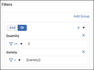
3. If the filter group requires additional filter expressions, expand the + list and select a column, then select a logical operator at the top of the filter group:

• And -- Data must satisfy all filter expressions in the group.
• Or -- Data must satisfy one or more filter expressions in the group.

4. Define additional filter expressions within the group as required.
5. If the filter set requires another group of filters:

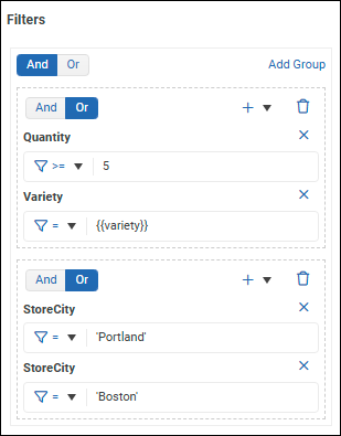
• Select Add Group and then, at the top of the filter editor, select a logical operator to apply to the set of groups:
  • And -- Data must satisfy all groups.
  • Or -- Data must satisfy at least one of the groups.
• Within the new group, define filter expressions and select a logical operator if the group contains multiple expressions.

6. Continue to add and define filter groups as required. The following example has two groups.

Formatting Tab#

The Formatting tab enables you to define the default visual appearance of cells in the report. These defaults can be overridden by individual column formats.

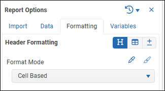
To format report contents:

1. Select an icon to select the type of cells to configure:

• -- Header cells
• -- Data cells
• -- Subtotal cells

2. From the Format Mode list, select one of the following:

• None -- No formatting defaults are applied.
• Automatic -- Standard Reportworq formatting.
• Cell Based -- Any Excel formatting you apply to a cell of the selected cell type within the report will be applied to all cells of that type. For example, if you are formatting data cells, you can apply formatting to one data cell and when you refresh the report, all data cells in the report will be formatted to match.
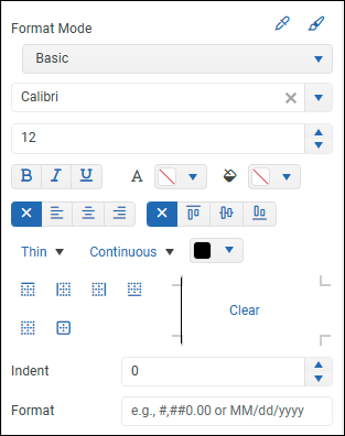
• Basic -- Enables you define formatting using tools that appear within the add-in, as shown below:
• Style -- Applies formatting based on a named style from Excel.
• Range -- Applies formatting to match the formatting of cells in the specified cell range.

Variables Tab#

The Variables tab lists all Reportworq variables applicable to the report.

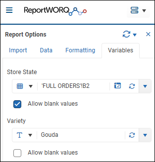
Each variable is part of a filter definition for a filter applied at the report level, the column level, or in the underlying reporting model. Only data that satisfies all filters is included in report output.

Note: All variables must be assigned values in order to run the report or refresh the report.

To assign a value to a variable:

1. From the list, select the type of variable value, either Text or Cell Range:

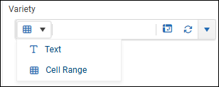
• Text -- A single text value.
• Cell Range -- A cell reference to a single cell that contains the value. If you specify a cell range, the value from the top left cell of the range will be used. Tip: You can create a report parameter in a Reportworq Job to populate the cell. The same parameter can then be used as the criterion for burst report iterations.

2. If the value is a text value, type the text in the box.
3. If the value is a cell reference, type the cell location in the box or select the cell selection icon and then select the cell on the worksheet.
4. Clear or select the Allow blank values checkbox:

• Clear -- A variable value must be provided here.
• Selected -- If no variable value is provided here, the default value from the underlying reporting model is used.

Editing Column Options#

Column options define which columns and data appear in the report, and the visual appearance of each column's contents.

Note: For options that can be set at both the report level and at the column level, column level settings override those set at the report level.

To access column options:

• From the Manage Reports view, select the report name.

The Columns list appears. The following example lists columns for a report named Products.

Choosing Fields#

Columns are based on data fields from the underlying Datasource. You can choose which fields are made available to be displayed in report columns. By default, all fields are available.

To exclude a field from the report:

1. Select the fields icon. The Choose Fields list appears.
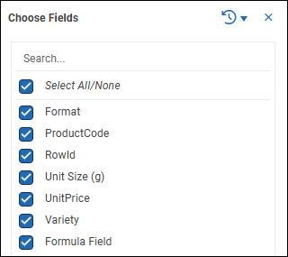
2. Deselect the field.
3. Close the Choose Fields list.

Displaying and Reordering Columns#

In the columns list, you can show or hide individual columns to control which ones appear in report output, and you can arrange the column order.

To show or hide columns:

• Select the columns you want to display in the report output. The open eye icon indicates that the column is displayed in the report. The closed eye icon indicates that the column is not displayed in the report. Note: Only columns that are based on available data fields appear on the list. For more information, see Choosing Fields. Tip: Hidden columns are still available for filter references.

To reorder columns:

1. Hover over the dots beside a column that you want to move. The drag icon appears.
2. Select and drag the column to the desired position in the list.

Formatting Columns#

Each column is formatted individually. Format options include:

• Header options -- Header text, grouping, and sectioning.
• Data options -- Sorting, aggregating, and filtering data.
• Formatting options -- Visual appearance of headers, data, and subtotals.

Note: Formatting applied at the column level overrides formatting applied at the report level.

To access the format options for a column:

• In the list of columns, select the arrow to the right of the column name. Format Options appear on three tabs (Header, Data, and Formatting.)

Header Options#

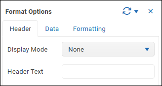
The Header tab contains the following options:

• Display Mode -- Enables you to group or section data based on the current column. You can set grouping and sectioning on multiple columns in the same report. The options are as follows:
  • None -- The report is not modified.
  • Group -- Where the data value for the current column is identical in multiple consecutive rows, only one instance of the value is displayed. In the following example, the Group display mode is applied to the Format column. 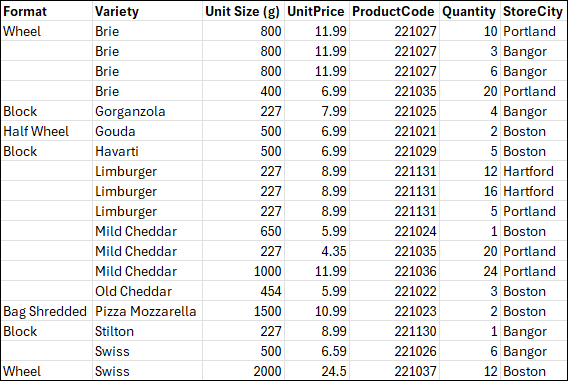Tip: To eliminate unwanted borders for empty cells and centre the values upon which the groups are based, select Merge grouped cells. Tip: You can sort the current column so that for each data value, all rows that have that value are displayed together, as shown below. Sort Mode options are available on the Data Tab.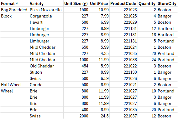
  • Section -- The report is divided into sections based on values from the current column. All rows that contain a given value are displayed in one section. In the following example, the Section display mode is applied to the Format column. 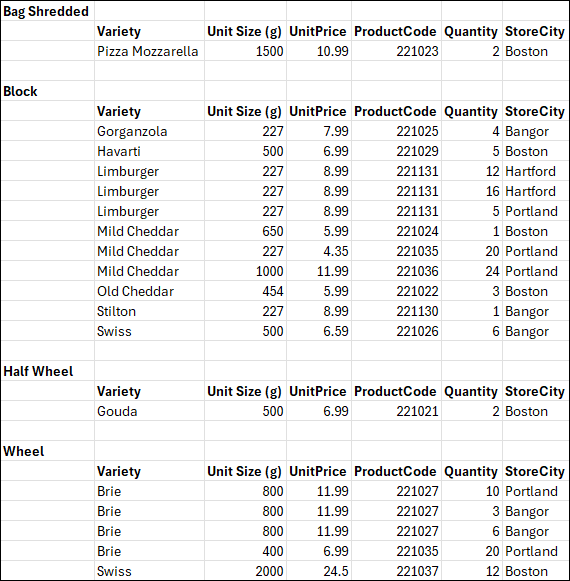When you section a column, additional Section Sorting and Layout Options appear: The
    • Display section in separate column -- Current column values, upon which the sections are based, are displayed in a separate column. When not selected, they are displayed above the first column.
    • Merge cells in section row -- Eliminates unwanted borders for empty cells.
    • Show totals for aggregate fields -- Enables the display of aggregate values for columns that have aggregation configured. Aggregate options are available on the Data Tab. If any columns in the report are grouped or sectioned, they must be configured to show totals for aggregate fields, on the Header tab of their Column Options. On the Data tab of the Report Options, the Show totals for aggregate fields option must be selected.
    • Auto outline section -- Creates an outline in Excel, with each report section as a collapsible Excel group.
    • Insert blank row -- Inserts a blank row between sections.
    • Insert page break -- Inserts a page break between sections.
• Header -- Enables you to define the header text.

Data Options#

The Data tab contains the following options:

• Sort Mode -- Enables you to sort rows based on the current column. 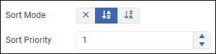If you want to apply nested sorting to multiple columns, set the Sort Priority for each sorted column. Lower-numbered sorting takes precedence. Do not assign the same sort priority to multiple columns.
• Aggregate -- Enables you to aggregate data values for the current column. 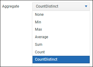Aggregate options are as follows:
  • None -- Values are not aggregated.
  • Min -- The lowest value is displayed. Applies to numerical values only.
  • Max -- The highest value is displayed. Applies to numerical values only.
  • Average -- The average value is displayed. Applies to numerical values only.
  • Sum -- All values are added, and the result is displayed. Applies to numerical values only.
  • Count -- Displays the total number of values, including repeated values. Applies to text values only.
  • Count Distinct -- Displays the number of unique values. Applies to text values only.
• Filters -- Enables you to define data filters for the current column. Rows that do not meet all filter criteria are excluded from reports. Tip: You can also define a set of filters at the report level, on the Data tab of Report Options.

To define filters for the current column:

1. Select Add Filter.
2. Define the first filter expression by selecting a comparison operator and specifying a test value. In the following example, the filter requires the data value to be greater than or equal to 5. If the test value is text, enclose it in single quotes as shown below: The test value can be a variable. In the following example, the test value is a variable named myVar.
3. If additional filter expressions are required, select Add Filter and then select a logical operator:

• And -- Data must satisfy all filter expressions in the set.
• Or -- Data must satisfy one or more filter expressions in the set.

4. Define additional filter expressions as required.

Formatting Options#

The Formatting tab enables you to define the visual appearance of cells for the current column.

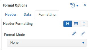
To format column contents:

1. Select an icon to select what type of cells to configure:

• -- Header cells
• -- Data cells
• -- Subtotal cells

2. From the Format Mode list, select one of the following:

• None -- No formatting is applied to the column.
• Inherit -- Formatting is inherited from the report-level format options.
• Automatic -- Standard Reportworq formatting.
• Cell Based -- Any Excel formatting you apply to a cell of the selected cell type within the column will be applied to all cells of that type. For example, if you are formatting data cells, you can apply formatting to one data cell and when you refresh the report, all data cells in the column will be formatted to match.
• Basic -- Enables you to define formatting using tools that appear within the add-in, as shown below:
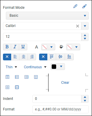
• Style -- Applies formatting based on a named style from Excel.
• Range -- Applies formatting to match the formatting of cells in the specified cell range.

Columns Based on Unmapped Fields#

The underlying reporting model may include fields that are not mapped to data fields from the datasource. By default, these appear in your report as columns that have a header but no data.

You can enter an Excel formula into the top non-header cell. When the report is refreshed, the formula is applied and is propagated to all non-header cells in the column.

If you want to use the column as an empty spacer column instead, you can edit the column's Formatting Options to replace the header text with spaces. Column width is determined by the number of spaces you type.

Alternatively, if you do not want to display the column, you can hide it in the column list, or exclude its data field from the report entirely.